Overcome Challenges in LNP Vector Analysis
eBook
Last Updated: November 25, 2025
Credit: Malvern Panalytical.
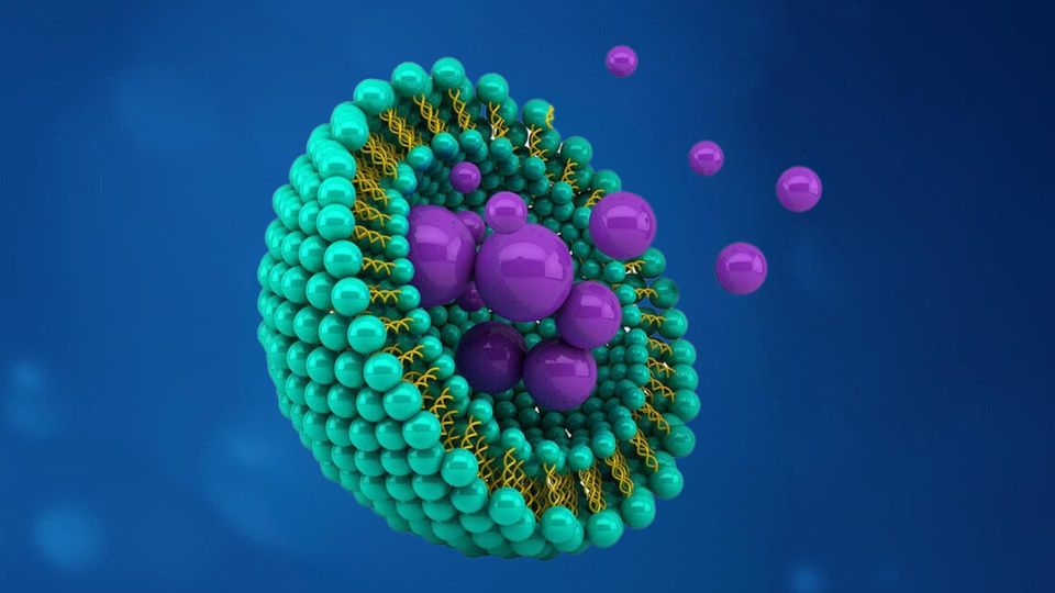
Lipid-based nanoparticles (LNPs) efficiently deliver therapeutic RNA payloads and can be rapidly scaled up through cell-free production processes. However, their complex structure presents analytical challenges, requiring precise measurement and control of attributes like size, concentration and thermal stability.
The analytical techniques that formulation developers and manufacturers typically use to characterize LNPs often fall short. They can leave users struggling to make confident decisions, hindering progress and slowing the route to market.
Download this eBook to discover how to overcome these obstacles with:
- Robust size, polydispersity, concentration and thermal stability measurements
- Data to help you interpret vector composition and quantify payload
- Information to help you design safe and effective LNPs for vaccines and therapeutics
Accelerating LNP Therapeutics
Your Guide to Smarter Analytics
2ND EDITIONContents
Introduction 3
Chapter 1: Characterizing LNP size,
polydispersity, and concentration 4
Size 5
Polydispersity 12
Concentration 14
Section summary 15
Chapter 2: Characterizing vector surfaces 16
Surface charge: zeta potential determination by ELS 17
Section summary 19
Chapter 3: Investigating thermal stability 20
Measuring thermal stability with differential scanning calorimetry (DSC) 21
Key considerations when using DSC 24
Section summary 25
Your route to analytical excellence
Optimizing LNP vector characteriztion
with the right tools 26
Featured & related products from Malvern Panalytical 27
Accelerating LNP therapeutics: Your guide to smarter analytics 2Introduction
Lipid-based nanoparticles (LNPs) hold great promise for the
treatment, cure, and prevention of a range of challenging
medical conditions — from genetic diseases to cancers.
Not only do these vectors enable the efficient delivery of
therapeutic payloads such as RNA, but (unlike viral vectors),
they can also be manufactured using cell-free production
processes with the potential for rapid scaling.
However, LNP therapies are analytically challenging to
develop and manufacture, owing to their intrinsic structural
complexity (Figure 1). Developers must accurately measure
and carefully control a range of key attributes to determine
their stability, and guide and inform product design,
production process optimization, and release specification.
Some of the key attributes of LNPs include:
• Size
• Polydispersity
• Concentration
• Zeta potential
• Higher order structure (HOS)
• Thermal stability
Critically, traditional techniques used for the
characterization of earlier, more established therapeutic
modalities, such as monoclonal antibody therapies,
are often not suitable for the complexity or pace of
development when it comes to novel LNP-based therapies.
As such, developers urgently need a suite of fit-forpurpose orthogonal analytical techniques that are
complementary to traditional approaches. Such tools
can help guide and optimize everything from vector design
through formulation development and manufacturing, to
quality control, enabling more confident decision-making
for faster delivery of better medicines to patients in need.
Figure 1: Illustration of a typical messenger RNA (mRNA)-LNP
complex (DSPC = distearoylphosphatidylcholine).
Cationic lipid DSPC PEGylated lipid Cholesterol mRNA
By reading this eBook, you’ll discover:
• How to get insights into the key
attributes of LNPs
• Robust, orthogonal analytical tools
that can help you to measure LNPs
with confidence
Accelerating LNP therapeutics: Your guide to smarter analytics 3Chapter 1: Characterizing LNP size,
polydispersity, and concentration
Accelerating LNP therapeutics: Your guide to smarter analytics 4Size
LNP vector size is a critical attribute for the function of LNP-based
therapies, as it can determine tissue penetration (and, therefore, in
vivo efficacy). In addition to giving you insight into LNP function,
accurately measuring the size of your LNP vectors can also help
you identify potential instability in your sample (typically displayed
as aggregation or a change in particle size, for instance) due to external
stresses, such as storage conditions or processing steps.
Size measurements are used across all stages of creating a new LNPbased therapy, from early development, through to process and
formulation development, process control, and final batch release.
Sizing up your LNPs: available tools & techniques
For LNP-based therapeutics, there are a number of size-measuring
analytical techniques, which cover a wide range of particle sizes -
namely single angle Dynamic Light Scattering (DLS), Multi-Angle
Dynamic Light Scattering (MADLS), and nanoparticle tracking
analysis (NTA). These techniques cover a wide particle size range.
Accelerating LNP therapeutics: Your guide to smarter analytics 5Small Particles
Intensity
Time
Intensity
Time
Intensity Intensity
Time
Time
Intensity
Time
Avalanche Large Particles
photodiode
detector (APD)
Digital signal
processor
(Correlator)
Small Particles
Cumulants analysis:
Z-average
Polydispersity index (Pdl)
Particle size distribution
(non-negative least squares
(NNLS) analysis):
Peak size, width and area
Large Particles
Laser
Cuvette
containing sample
Side scatter
detection angle
ZS Advance Lab/Ultra
Back scatter
detection angle
Forward scatter
detection angle
ZS Advance Pro/Ultra
ZS Advance Pro/Ultra
Figure 2: Diagram showing how dynamic light scattering works.
Dynamic Light Scattering (DLS)
DLS is a non-invasive, well-established technique for measuring the size and
size distribution of molecules and particles dispersed or dissolved in liquid
(Figure 2). In DLS, a light source illuminates a dispersion of particles. The
particles then scatter a fraction of the light in all directions, with some of
this scattering detected at a single, specified angle. Analyzing the scattering
intensity fluctuations gives the velocity of the Brownian motion, which is then
used to calculate the particle size using the Stokes-Einstein relationship.
With the latest technology, DLS can detect particles ranging from 10s of µm to
1 nm and below, meaning it can help you reliably measure even the smallest
mRNA-LNPs (which typically range from ~50–150 nm).
One critical benefit of DLS is its wide concentration range, which is a particular
advantage for LNPs as they can often occur in very high concentrations.
While DLS has the lowest resolution of the three sizing techniques discussed
here, it is accurate, reproducible, fast, and requires limited method development.
As such, analysts often use DLS as a rapid screen for sample degradation
or aggregation, providing an indication of whether deeper investigation of your
LNP vector’s size is needed.
What’s more, DLS also uses minimal sample volumes (~1 uL) non-destructively,
meaning you can preserve your precious samples and re-use them in other assays.
However, you should be aware of one critical disadvantage when it comes to
single-angle (backscatter) DLS: larger aggregates tend to scatter more light in
the forward angle, meaning that it can be difficult to detect the presence of LNP
aggregates. For this reason, you should always quote the scattering angle used
to obtain your DLS result.
Briefly how it works!
Accelerating LNP therapeutics: Your guide to smarter analytics 6Single Angle DLS
Three angles give three different broad distributions
Correlation Coefficient (g1-1)
Time (µs)
0
0.01 0.1 1 10 100 1e+03 1e+04 1e+05 1e+06 1e+07 1e+08
Size (d.nm)
0.1 1 10 100 1e+03 1e+04
0.2
0.4
0.6
0.8
1
Intensity (Percent)
5 0
10
15
20
25
1.2
Correlation Coefficient (g1-1)
Time (µs)
0
0.01 0.1 1 10 100 1e+03 1e+04 1e+05 1e+06 1e+07 1e+08
0 100 200 300 400 500 600 700 800
45 (Mie)
90 (Mie)
173 (Mie)
900 1000
Diameter (nm)
0.2
0.4
0.6
0.8
1
Normalised Scattering Per Particle (Mie)
1e-08
1e-06
1e-04
1e-02
1e+00
1.2
Intensity (Percent)
Size (d.nm)
0
0.1 1 10 100 1e+03 1e+04
8 6 4 2
10
12
MADLS
One accurate and more resolved distribution from the same data
Multi-angle dynamic light
scattering (MADLS)
While DLS works by measuring
samples at a single detection angle,
MADLS measures samples at
multiple angles, offering improved
resolution as well as angleindependent particle size
distribution (Figure 3).
MADLS, therefore, has several
advantages relative to single angle
DLS. First, it provides a more
accurate representation of the
different populations present in the
sample, and a higher resolution
size determination of multi-modal
samples (Figure 4). It can also
consistently detect low numbers of
larger aggregates (which are inherently
harder to detect with single angle
DLS, as discussed above).
Figure 3: Comparison of Single angle DLS and MADLS. By combining the correlation data from several scattering angles with Mie theory, MADLS
provides a single, more representative, and better-resolved size distribution relative to single angle DLS.
Accelerating LNP therapeutics: Your guide to smarter analytics 7MADLS
NIBS
16
14
12
10
8 6 4 2
10 100 1000 10000
Size Diameter (nm)
Intensity (%)
0
Like DLS, MADLS can detect even the smallest
LNPs, with a detectable size range of 10 µm to
1 nm and below.
A key consideration for using MADLS is that you
need to know the refractive index and absorption
of your sample material and dispersant. Without
the correct values, the MADLS algorithm will
fail to converge on the true solution, giving you
inaccurate results. Since RNA can change the
refractive index of your sample, you need to know
if your samples contain RNA or not. To do this,
you can either calculate the refractive index from
a RiboGreen assay, or you can calculate it from
compositional analysis data.
Figure 4: MADLS reveals a second population (shoulder) alongside the NIBS measurement, providing higer
resolution overall
Accelerating LNP therapeutics: Your guide to smarter analytics 8Image Capture Analyse Data
NTA doesn’t require any knowledge about material constants such
as RI or absorbance of the particles - orthogonal technique
Polydispersity
Size
Flourescence
Number or concentration
“Relative Light Intensity”
Nanoparticle tracking analysis (NTA)
Nanoparticle Tracking Analysis (NTA) utilizes the
properties of both light scattering and Brownian
motion to obtain the nanoparticle size distribution
of samples in liquid suspension (Figure 5).
For this technique, particles in liquid suspension
are loaded into a sample chamber, which is
illuminated by a laser beam. Particles in the path
of the beam scatter the light, which is then
collected by a microscope and viewed with
a digital camera.
The camera captures a video of the individual
particles moving under Brownian motion, with
software analyzing many particles individually
and simultaneously, particle-by-particle. By using
the Stokes Einstein equation, NTA software then
calculates the hydrodynamic diameters of the
particles.
Tracks particles in real time and reports on several characteristics
Figure 5: Diagram showing how NanoSight Pro obtains
a particle size distribution.
Accelerating LNP therapeutics: Your guide to smarter analytics 910 10
0.0
5.0e+5
1.0e+6
1.5e+6
2.0e+6
2.5e+6
3.0e+6
5 0
10
15
20
100 100
Size Diameter (nm)
Concentration (p/mL)
Size Diameter (nm)
Intensity (%)
1000 1000
MADLS
NIBS NTA
Most importantly NTA offers much higher
resolution than MADLS, meaning that it is a
superior technique for analyzing polydisperse
LNP samples (Figure 6). With real-time monitoring
capabilities, NTA can also monitor subtle changes
in the characteristics of your LNP populations,
which you can confirm with visual validation. One
example is its ability to detect low levels of closely
spaced aggregate populations—often critical for
the early identification of suboptimal buffer or
storage conditions that fail to protect samples
from environmental or process-related stresses—
thereby supporting scientists in developing longterm stability strategies.
Similar to MADLS and DLS, NTA also uses very
small sample volumes (1 µl, before dilution), nondestructively, and with little sample preparation
needed.
However, NTA has a few downsides that you
should be aware of. First, NTA cannot detect
LNPs below 30 nm. NTA is also less sensitive
than either DLS or MADLS in detecting small
populations of larger aggregates, as it is a
numbers-based technique. However, this is where
the techniques complement one another: NTA
offers unique visibility into subtle changes in
closely spaced sample populations—something
DLS and MADLS often struggle to resolve.
Additionally, because NTA typically requires
significant sample dilution, analysts should
verify sample stability, for example by measuring
replicates over an extended period.
Figure 6: Comparison of size distribution measurements of an mRNA-LNP sample using DLS (left, blue), MADLS (left, red),
and NTA (right), where NTA demonstrates superior resolution to both DLS and MADLS.
Accelerating LNP therapeutics: Your guide to smarter analytics 10Automating dynamic light scattering
workflows
Sample Assistant, the robotic accessory for Zetasizer
Advance, boosts lab efficiency while delivering highquality, reproducible data.
• Maximize throughput by fully automating sample
changes
• Free up your team to focus on higher-value tasks and
analysis
• Run size and zeta potential measurements
automatically—with zero risk of crosscontamination
• Switch between measurement types from a
single tray, with no manual reconfiguration
• Stay on track with an intuitive workflow that
simplifies maintenance and minimizes downtime
Choosing the right tool for the job: key considerations
As we’ve seen, several tools are available for measuring the size of your
LNP vectors. To ensure you make the appropriate choice, keep in mind
the following factors:
• Particle size and polydispersity
NTA struggles to measure particles below 30 nm, whereas advanced DLS
and MADLS systems can measure particles below 1 nm. When it comes to
polydisperse samples, MADLS has superior resolving power relative to DLS,
but NTA has the best resolving power
• Concentration range
See the section on concentration range (page 14) for more detail on the
accessible concentration range of MADLS, NTA and SEC-LS, which provide
valuable measurements across a wide range of concentrations
• Stage of development and sample volume available
Both DLS and MADLS require only small amounts of samples (~1 μl for DLS
and 20 μl for MADLS) making the techniques a good choice for earlier stages
of development (where only smaller amounts of samples may be available).
While NTA requires ~ 1ml of samples, this is heavily diluted, requiring only 1 µl of
undiluted LNP solution
• The specific question you want to ask of your sample
For instance, if you want to see if your sample has aggregated (but don’t
require deeper information about the nature of these aggregates), DLS
can be a rapid route to a reliable answer. If, on the other hand, you wish
to understand what aggregates have formed, higher resolution techniques
such as MADLS or NTA may be the best option
Accelerating LNP therapeutics: Your guide to smarter analytics 11Polydispersity
Polydispersity is a measure of the heterogeneity (in terms of particle
size) of a sample. It’s an important attribute to measure, as it can
help you assess sample stability throughout development and
manufacture, as well as help track process reproducibility and
monitor changes in size distribution due to environmental stress.
Importantly, when investigating sample polydispersity, you can look at
either the polydispersity of the whole sample (which is used to describe
the presence of aggregates or agglomerates), or the polydispersity of
an identified population among many populations in the same sample.
Critically, different analytical tools will provide different measures
of polydispersity.
Tools & techniques
The tools you can use to measure LNP sample polydispersity are the
same as those used to measure size: DLS, MADLS, and NTA with in-line
light scattering detectors. Below we discuss which tool provides which
measure of polydispersity, how the measure is calculated,
and how they should be interpreted.
The polydispersity index (DLS)
The polydispersity index (PDI) is a useful and common parameter for measuring
sample heterogeneity. It’s a dimensionless measure that describes the broadness
of the sample size distribution, and ranges from 0.01 (perfectly uniform) to >1 (highly
polydisperse) (table 1). (The PDI is calculated from the DLS cumulants analysis method)
The Span (DLS, MADLS, and NTA)
The Span is another common and useful measure of sample polydispersity,
indicating how far the 10% and 90% points of the distribution are from each other,
normalized with the distribution midpoint.
(Span = (D90 – D10)/D50)
You can calculate the Span from DLS and MADLS data (but you’ll need to
transform this data to volume distributions), or from NTA size distributions. The
closer the Span value is to 0, the more monodisperse your sample population.
Polydispersity parameter Definition Distribution type
‘Monodisperse’ ‘Polydisperse’
Uniform Narrow Moderate Broad
PDI (DLS)
(distribution standard
deviation/distribution
mean)^2
0.04 0.0–0.1 0.1–0.4 >0.4
Table 1: Values of different classes of sample dispersity.
Accelerating LNP therapeutics: Your guide to smarter analytics 12Considerations
Given that polydispersity is calculated using the same instruments
(and uses the same measurements) as when characterizing particle size,
the considerations for which tool is best are mostly the same — namely
that your LNP is in the detectable size and concentration range, and that
you have sufficient sample to meet the instrument’s requirements.
It is also worth noting that polydispersity measurements will be
inherently more variable than size measurements, given that the
smallest variation in size polydispersity is not necessarily reflected in
the average size value.
Important tip
There is no one-size-fits-all approach when it comes to
deciding on the best parameter to track the polydispersity
of your LNPs or determining an acceptable polydispersity
level for your sample. Both ultimately depend on the type of
particles you’re working with, as well as their intended end
use, route of uptake, and fate in the body. As such, you’ll need
to use a case-by-case approach.
Accelerating LNP therapeutics: Your guide to smarter analytics 13Concentration
Concentration is another important attribute to measure when
characterizing and tracking LNP therapies. Though not as commonly
used (the methodologies used to measure concentration are still
considered immature relative to particle sizing techniques), exploring
concentration during the design, formulation, and processing of your
LNP therapy is highly beneficial, as it helps
to monitor yield.
Tools & techniques
As with size and polydispersity measurements, you have multiple
tools at your disposal for measuring the concentration of LNP vectors,
ranging from mass-based techniques (measured in mg/ml) to numberbased techniques (measuring the number of particles in a given
volume of sample).
MADLS and NTA can provide valuable particle-based concentration
measurements across a wide range of concentrations, offering
measurements that are orthogonal to mass-based techniques.
The accessible concentration ranges of each technique are
detailed in Table 2.
Importantly, as can be seen from Table 2, NTA can offer measurements
complimentary to MADLS, overlapping with but also extending the detectable
concentration range by an order of magnitude at the lower end. It is also worth noting
that larger samples will show non-linear behavior at the highest concentrations, owing
to increased scattering effects of larger particle sizes at higher concentrations.
Technique Accessible concentration range Accessible size range
Nanoparticle tracking analysis
(NTA)
Optimal concentration range of
~10^7 – 10^9 particles/mL 50-100 nm
Multi-angle dynamic light
scattering (MADLS)
From 10^8 – 10^13 particles/mL.
Range is determined by the amount of
light scattered (directly related to vector
size and refractive index). Larger vector
sizes = increased scattering = lower
accessible concentration.
<1 nm to 10 µm
Table 2: Comparison of the accessible concentration ranges of NTA and MADLS.
Considerations
Considerations for choosing the right concentration-measuring
tools are largely the same as for measuring sample size — i.e., the
size of your particles, whether you have enough sample (in terms of
concentrations of particles), and how detailed you need your analysis
to be (MADLS offers a quick, rough particle concentration screen),
while NTA offers more detailed results.
Accelerating LNP therapeutics: Your guide to smarter analytics 14Section summary
Size, polydispersity, and concentration are key attributes to define and monitor when it comes to LNP-based therapy design, development, and manufacture.
LNP vector size
• A critical determinant of LNP vector
tissue penetration, and can indicate
sample instability
• DLS, MADLS, and NTA offer accurate and
reliable ways to measure LNP size across a
range of particle size ranges, and with different
resolutions (see table on page 14)
• Choosing the right tool depends on
several considerations, including the size
and polydispersity of your LNP samples,
sample concentration, available sample
volume, and what you are looking to find
out about your sample
LNP vector polydispersity
• Provides important insights into LNP sample
stability and process reproducibility
• DLS, MADLS, and NTA can all be
used to effectively measure polydispersity,
although in different ways
• Optimal tool (and therefore parameter)
choice ultimately depends on the same
considerations as when measuring particle size
(the tools are the same)
LNP vector concentration
• An important attribute to track, informing
you about yield
• MADLS and NTA provide valuable particlebased concentration measurements across a
wide range of concentrations,
and offer measurements orthogonal to
mass-based techniques (see table on page 14)
• Technique choice depends on the size of
your LNPs, the amount of sample you have
available, and how detailed you need your
analysis to be (MADLS offers a quick screen
while NTA can access lower concentrations
with more precision for polydisperse samples)
Accelerating LNP therapeutics: Your guide to smarter analytics 15Chapter 2: Characterizing vector surfaces
Accelerating LNP therapeutics: Your guide to smarter analytics 16Zeta potential a particle/molecule acquires in a particular medium.
- +
Voltage
Electrode Electrode
Capillary
- +
Slipping plane
Electrical double layer
Stern layer Diffuse layer
Figure 7: Diagram showing how electrophoretic light scattering system works with zeta potential or indication of particle in a solution.
Zeta potential (indicative of surface charge in a
certain environmental condition e.g. pH/salt) is a
key attribute in the development of LNP therapies.
It is one of the most important determinants of
an LNP’s solubility and interaction with cellular
membranes. (Importantly, the optimal zeta
potential value depends on your target tissue).
Knowledge of the surface charge can therefore
help you predict the in vivo fate and activity of your
LNP therapy.
Additionally, surface charge information
can offer insight into its surface chemistry, as
well as its colloidal stability in solution and its
tendency to form aggregates in solution
(and any modifications it may undergo).
Several factors can influence the measured
zeta potential:
• Changes in pH
• Ionic strength
• Concentration of other components
in the solution (such as additives,
coagulants, and surfactants)
As such, to ensure reproducible zeta potential
measurements, you should always report the
sample buffer you’ve used, as well as the
conductivity that the instrument measured
for the zeta potential value.
Zeta potential determination by ELS
Electrophoretic light scattering (ELS) is a key tool that you can use to measure the zeta potential of your LNP samples.
The fundamental physical principle of ELS is electrophoresis (Figure 7). A dispersion is introduced into a cell containing
two electrodes, and an electrical field is applied across them. Particles with a net charge migrate towards the oppositely
charged electrode with a velocity (known as the electrophoretic mobility) related to their zeta potential. A laser
is passed through the bottom of the cell, with the charged particles producing scattered light that is frequency shifted
in proportion to their velocity. By detecting the frequency shifts, we can then calculate the zeta potential.
When it comes to LNP samples, ELS is most often used to validate the apparent surface charge of your LNPs —
for example by measuring the zeta potential of your LNPs in PBS, or a 10x diluted version of your sample,
to evaluate your LNP formulations (e.g., for stability, predicted uptake efficiency in target tissues).
Electrophoresis = movement of
a charged particle relative to the
liquid it is suspended in under the
influence of an applied electric field
Zeta potential =
electrical potential at the slipping plane
Zeta potential or indication of particle charge in a solution
Accelerating LNP therapeutics: Your guide to smarter analytics 17Figure 8: Overview of the DBM for ELS measurements. With the DBM, gel
electrophoresis loading pipettes are used to insert a small ‘plug of sample’ into the
cell.
A key challenge of measuring zeta potential:
high-conductivity samples
High conductivity samples pose significant challenges when it comes to measuring
zeta potential, as they can lead to inaccurate measurements. This is important, as LNP
therapies are prepared in physiological buffers, which are high conductivity.
High-conductivity samples interfere with accurate zeta potential measurements in four ways:
Joule heating effects, electrode polarization, electrode degradation, and sample degradation
(simply applying a voltage across a high-conductivity sample can cause it to aggregate).
Overcoming challenges of high-conductivity
samples with the diffusion barrier method
To ensure your zeta potential measurements are accurate and precise when working
with high-conductivity samples, you can use the diffusion barrier method (Figure 8),
which mitigates the above-mentioned adverse effects.
The diffusion barrier separates the particles in your sample from the electrodes by
inserting a small ‘plug’ or aliquot (~20–100 ul) of sample into a folded capillary cell that
already contains the same buffer that the sample is prepared in. The sample is therefore
isolated due to the physical distance between the sample and the electrodes. The time
it takes for the particles to diffuse to the electrode is significantly longer than the
duration of the measurement itself.
Since the sample is not directly in contact with the electrodes, sample integrity is maintained,
and electrode degradation is minimized. Furthermore, the diffusion barrier method (DBM)
also reduces the amount of sample required for zeta potential measurements.
Traditional
fill method
~750 ul
Diffusion barrier
fill method
~20-100 ul
Patented by
Malvern Panalytical
Assessment of charge differences between formulations
Accelerating LNP therapeutics: Your guide to smarter analytics 18Important tip
While the diffusion barrier method can mitigate
the risk of sample degradation, ELS is still an
invasive measurement. Accordingly, to ensure
sample integrity is not adversely impacted by the
measurement, you should measure the size of your
sample both before and after ELS measurements (for
example, using five repeat DLS measurements).
Section summary
Zeta potential is an important attribute of LNPs that can indicate
colloidal stability and help predict cellular membrane interactions
• Zeta potential can also give insight into the surface chemistry of LNPs
• Electrophoretic light scattering (ELS) is a valuable tool to measure the zeta potential
of your LNP samples, helping you to evaluate the stability of your formulations and
optimize target tissue uptake
• High-conductivity samples can make accurate and precise zeta potential measurements
challenging - the DBM technique helps you overcome this
• Since ELS is an invasive technique, analysts should measure the particle size
of their samples before and after to see if sample degradation has occurred
Accelerating LNP therapeutics: Your guide to smarter analytics 19Chapter 3: Investigating thermal stability
Accelerating LNP therapeutics: Your guide to smarter analytics 20T=20°C
Folded
T=90°C
Unfolded
Temperature (°C)
T
m
N
D
Excess heat capacity (C
p
)
20 40 60 80 100
H
Area= cal
T
onset
T
1/2
Figure 13: Schematic of a typical DSC instrument.
LNPs are non-covalent assemblies of lipids and
mRNA with mRNA being a crucial structural
component. Structure and structural stability
are key properties ensuring desired function
and safety of LNP vectors and their cargo.
Temperature change is a common stress factor
for LNP-based therapies throughout production,
storage, and application. Being able to measure
and compare thermal stability profiles helps you
to assess the inherent structural stability
of LNPs and their mRNA cargo.
Such insights can help you track changes
between batches and stress conditions, helping
you know if you are producing the same higher
order structure, or whether those particles change
(or have changed) structurally due
to certain stressors.
Differential scanning calorimetry (DSC) is a valuable
and well-established tool for monitoring the thermal
stability and thermally induced transitions of
biomolecules and biomolecular assemblies including
lipid-based delivery vectors and nucleic acids.
How does DSC work?
Broadly, DSC works by measuring the heat change associated with a sample’s structural transitions
when heated at a constant rate.
The thermal core of a DSC system consists of two cells — a reference cell, and a sample cell (Figure 13).
The device is designed to maintain the two cells at the same temperature as they are heated.
To perform a DSC measurement, you must first fill a reference cell with buffer and the sample cell
with the sample solution. The instrument heats these at a constant scan rate. The absorption of heat
that occurs when a molecule undergoes a structural transition causes a temperature difference (ΔT)
between the cells, resulting in a thermal gradient across the Peltier units (or thermoelectric modules).
This sets up a voltage, which is converted into power and is used to control the Peltier to return
ΔT to 0°C.
Accelerating LNP therapeutics: Your guide to smarter analytics 21Cp (kJ/mol/K)
Temperature (°C)
-2.78E-4
-1.78E-4
-7.84E-5
2.16E-5
1.22E-4
2.22E-4
3.22E-4
20 40 60 80 100
Loaded
120
Empty vs loaded
Cp (kJ/mol/K)
Temperature (°C)
-2.31E-4
-1.31E-4
-3.11E-5
6.89E-5
1.69E-4
2.69E-4
3.69E-4
4.69E-4
5.69E-4
40 50 60 70 80 90 100 110 120
Different mRNA amounts
Empty
Figure 14: Illustration of mRNA-LNP thermograms.
DSC thermograms – what they can tell us about a sample?
The output of a DSC measurement is a thermogram (Figure 13), which provides multiple parameters
for describing the thermally induced transitions of samples:
• T
m (thermal transition midpoint): This is the so-called melting temperature of the sample, denoted
by an endothermic peak in the DSC thermogram. The higher the thermal transition midpoint, the
more stable the sample. Shifts in Tm can indicate structural heterogeneity
or degradation
• T
onset (thermal transition onset): The onset temperature of the first thermal transition event is an
important factor to consider. A lower Tonset means that molecules are more likely to unfold at this
temperature, which increases the likelihood of aggregates forming. By understanding the Tonset
of your sample, you can identify temperature ranges that will minimize the risk of aggregation and
maximize sample stability
• T
1/2 (the width of thermal transition at half-height): The T1/2 reflects the extent of cooperativity
of the thermal transition. The narrower the transition, the more cooperative it is
• Enthalpy change (∆H): The enthalpy change is the total energy spent in a thermal transition.
This is represented by the area under the thermogram and reflects the relative amount of native
biomolecule in your sample
• Higher order structure (HOS): In addition to these parameters, the entire thermogram shape
can give us a fingerprint of the molecule’s HOS. The HOS is a valuable descriptor that can help
inform you about the stability profile of your biomolecules during product characterization,
formulation, and comparability analysis
• Reversibility: While not a feature of the thermogram itself, the reversibility of thermal transitions
is another key aspect of structural transitions observed with DSC. Reversibility reveals the ability
of biomolecules to re-adopt their native structure upon cooling. Low reversibility is characteristic
of unfolding events accompanied by aggregation and/or chemical degradation
Accelerating LNP therapeutics: Your guide to smarter analytics 22Taking a deeper look at RNA with DSC
RNA is a structurally flexible molecule that can exist in a variety of primary, secondary, and tertiary
structures. These structural differences can have significant effects on function, as well as impacting
RNA-LNP complexation. By revealing information about primary and secondary structure (though
T
m values and HOS), DSC results can give us insights into the functional efficiency, stability and
degradation, modifications, and half-life of the nucleic acids and oligonucleotides in question,
helping you to design and select optimal mRNA variants for your therapies.
Thermogram parameters can also reveal information about solvent conditions and hybridization
efficiency (primarily through the Tm value). And, as with LNP vectors, you can also measure ΔH values
and explore the RNA’s HOS to understand structural heterogeneity and possible degradation.
Overall, DSC offers a high-throughput (although low resolution) option for structural analysis. DSC
traces can inform you about the sample structure in a broad range of concentrations and solution
conditions without being limited by high absorbance limitations and without hypo/hyperchromicity
artifacts. With this technique, you can better design and select mRNA-LNPs and their components,
identify the conditions beneficial to the structural stability of mRNA-LNP formulation, processing,
and storage, as well as complement and enhance physico-chemical characterization of your lipidbased delivery vectors.
Using DSC to characterize LNPs
and nucleic acids
When it comes to LNP-based therapies, DSC
can provide a wealth of information, from overall
thermal stability and the effect of drug loading on
thermal stability, to information about LNP phase
structure. By detailing the HOS of your samples,
DSC also allows you to compare batches of drug
substance and drug product, helping you ensure
you’re delivering the same product consistently.
It’s important to remember that while mRNALNP assemblies are complex, RNA itself is also
complex, and can impact therapeutic protein
expression. It is therefore important to explore
and characterize your RNA payload.
Accelerating LNP therapeutics: Your guide to smarter analytics 23Key considerations when using DSC
When studying samples as complex as LNPs, it is important
that you can get the best possible instrument performance —
high resolution and accurate output that you can rely on
for confident conclusions about thermogram features
and differences.
However, lipid formulations can lead to carry-over
effects, which can reduce the accuracy and resolution
of DSC traces.
To minimize the impact of these carry-over effects,
it is vital that you properly clean the DSC cell and
syringe between scans.
With most DSC instruments, you can soak DSC cells
and rinse syringes with detergent after each scan. But
this is not always sufficient to eliminate sample carryover
effects, especially if the cleaning procedure is carried
out manually.
Advanced DSC systems, however, allow you to soak
the syringe in detergent during scanning, as well as
fully automate the cleaning process, eliminating sample
carryover effects while also saving time (Figure 15).
Indeed, since cleaning takes place during measurements,
the instrument is ready for the next sample immediately
after the first measurement is finished.
Figure 15: Comparison of LNP sample carry-over effects with (left) and without (right) enhanced syringe cleaning capabilities.
• SCAN after each LNP sample
• Syringe clean* after each LNP sample
* New feature available with upgraded PEAQ-DSC software (BSL2 support)
Carry-over
DSC s/w pre V1.6
(no BSL2 cleaning enabled)
• Cell can be soaked in detergent
• Syringe can only be rinsed
DSC s/w post V1.6
• Cell can be soaked in detergent
• Syringe can soaked during scans
DP
Temperature (°C)
DP
Temperature (°C)
Enhanced cleaning for higher resolution DSC and LNPs
Accelerating LNP therapeutics: Your guide to smarter analytics 24Section summary
• Differential scanning calorimetry (DSC) is a valuable and wellestablished tool for monitoring the thermal stability and phase
behavior of biomolecules
• DSC thermograms reveal a wealth of information about
biomolecules, from thermal stability to higher order structure (HOS)
• DSC helps inform the design and selection of mRNA variants and
LNP vectors, identify optimal conditions for structural stability of
mRNA-LNPs during formulation, processing, and storage, and can
enhance physico-chemical vector characterization
• Critically, by revealing the HOS of your LNP therapies, DSC can aid
batch comparability analysis
• Analyzing lipid formulations with DSC can lead to carry-over effects.
However, some systems now feature enhanced and automated
cleaning capabilities (BSL2) that can eliminate this
Accelerating LNP therapeutics: Your guide to smarter analytics 25Your route to analytical excellence
Optimizing LNP vector characteriztion with the right tools
LNP delivery systems offer much promise for cell and gene therapies and novel vaccines.
Developing and manufacturing LNP-based therapies, however, is fraught with difficulty.
As an LNP-based therapy developer, you must overcome the challenges posed by the intrinsic
structural complexity of LNPs to reliably measure their critical quality attributes. Only then can
you optimally guide their development, enable consistent manufacture, and ensure safe delivery
to patients.
A suite of robust, accurate, and highly reproducible biophysical techniques is available to help
you to overcome these challenges and better characterize the critical quality attributes of your
LNPs — from size, polydispersity, concentration and stability, to surface charge and composition.
These tools offer powerful, complementary approaches to tracking the development and
manufacture of your LNP-based therapies, delivering deeper insights while also offering
opportunities to minimize sample use, save time, and reduce costs.
Ultimately, with the right suite of insightful biophysical analytical tools, you can carve a swifter
path to analytical success in a complex and competitive field.
Want to learn more about how you can better characterize your LNP-based therapies?
Then reach out to our team of analytical experts, or visit https://bit.ly/3ZtVEob.
Accelerating LNP therapeutics: Your guide to smarter analytics 26Featured & related
products from
Malvern Panalytical
Explore how Malvern Panalytical’s best in class analytical
instruments can help you understand the structure, stability
and affinity of your nanodrug delivery systems.
NanoSight Pro View here
Zetasizer Advance View here
MicroCal DSC range View here
Zetasizer Sample Assistant View here
Accelerating LNP therapeutics: Your guide to smarter analytics 27
Brought to you by

Download this eBook for FREE Below
Information you provide will be shared with the sponsors for this content. Technology Networks or its sponsors may contact you to offer you content or products based on your interest in this topic. You may opt-out at any time.
Experiencing issues viewing the form? Click here to access an alternate version